Excel Error 0xc000142 – Trouble Opening Microsoft Office 2016 Excel and Word “EXCEL.EXE Application Error. The application was unable to start correctly (0xc0000142)”
The Problem: Microsoft Office tried to update itself this morning and wouldn’t complete the process. Instead, Windows threw the error “EXCEL.EXE Application Error. The application was unable to start correctly (0xc0000142)”.
Fantastic. We can’t open Microsoft Excel/Word for a mail merge and a client deadline is approaching.
After some digging, the most common cause for this error is a corrupted or missing system file.
Another failed update for Microsoft and Windows 10 in 2020.
Here’s a few that have stopped/delayed production and rendered legacy printers useless (for a little while at least).
https://www.techradar.com/news/new-windows-10-update-fail-could-break-your-start-menu
https://www.windowscentral.com/windows-10-may-2020-update-common-problems-and-how-fix-them
The Solution: We are going to “Repair” the Windows Office installation.
1. Press your “Windows Key” on the left hand side of your spacebar and start typing “remove programs”.
2. Click “Add or Remove Programs” under “Best Match” in the Start Menu. Don’t worry. We are going to “Repair” the software instead of “Removing” it. A window labeled “Apps & Features” will open.
3. Scroll down to “Microsoft Office 365 – en-us” and click “Modify”.
4. A “User Account Control” window will pop up and ask permission to make changes to your device. Click “Yes”.
5. Another window will then ask “How you would like to repair your programs?”. Click “Quick Repair”. Wait for the process to complete.
After double-clicking Excel or Word, we are back in business! Hopefully this will save someone else the time and hassle.
Web Scrape Multiple Earnings Call Dates From Yahoo Finance Using Excel (No Coding Involved)
The Problem: Yahoo finance shut down their stock data API in 2017. We can no longer make GET requests for stock information from their API.
Investors, competitors, the media, and even procurement departments follow the earnings calls of publicly traded organizations.
We are looking to automate the retrieval of the upcoming earnings calls for many companies at once instead of looking up each ticker one at a time. That would take too long and the dates/times of the earnings calls are subject to change.
Wouldn’t it be great if we had a simple list of past and upcoming earnings call dates in a simple excel sheet?
We would be able to quantify the companies that typically post earnings early, on time, or late and score them accordingly. It could bring up valid questions about the companies health or commitment to compliance.
Download the Earnings Calls Web Scraper for Excel
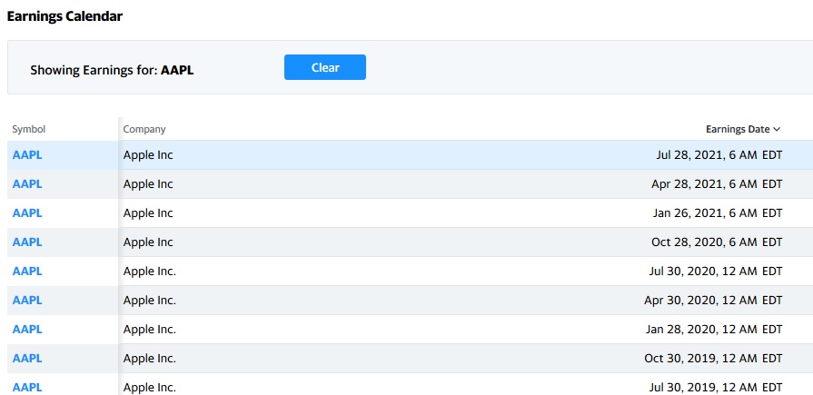
Here’s an example of the data we are trying to retrieve, but it’s only one company:
https://finance.yahoo.com/calendar/earnings/?symbol=AAPL
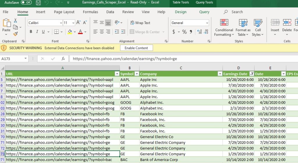
The Solution: Microsoft Excel has a Power Query feature that allows you to get data from a website. To take it one step further, we are invoking a custom function that passes in each individual ticker URL as a parameter.
This means we are making one request to Yahoo for each ticker URL.
https://finance.yahoo.com/calendar/earnings/?symbol=TSLA
This will result in one table for each ticker and then we will stack them like jenga blocks. Refresh the data to often in a short time (make to many requests) and Yahoo will limit your access. Yes, this happened to me.
I will go into the details of how this was built in a future post but for now I will explain how to use it.
Click “Data” in the toolbar and then “Queries & Connections”.
Right-click on “URL_List” then click “Edit”.
On the right hand side under “Applied Steps”, click “Source” and then the cog on the right.
Replace the ticker symbols on the end of the URL with your own. Feel free to add or delete records if needed. I choose the top 15 most followed tickers.
Click “OK” and then “Close & Load”.
Click “Refresh All” in the middle of the toolbar.
That’s it!
The sky is the limit with this list. You can create a dashboard in PowerBI to track upcoming or past earnings calls. Create your own metrics based on tardy earning reports and how often it happens. Or you can filter the list by categories/sectors and get a quick update as the earnings call dates approach. Times/dates are never set in stone and data from Yahoo is not as up to date as the Investor Relations page on a company website.
Calculate Semester Final Grade with VLookup, IF Function, and Conditional Formatting
A VLookup in excel is a function that “vertically looks up” a provided value and provides a corresponding lookup value to the right of it. VLookups are great for looking up additional information about a product based on a SKU number, UPC, or a unique ID number. They can also be used to lookup a grade letter based on the total points earned in a class.
In my spreadsheet below, I have created a sample grade sheet that assigns weights to each individual assignment. Download The Spreadsheet!
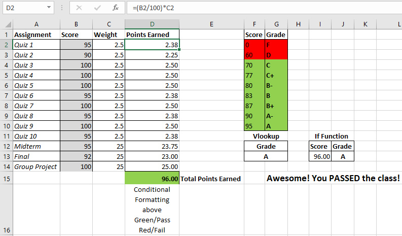
The midterm, final, and the group project are each worth 25% of the total grade. The remaining 25% of the total grade is divided among 10 quizzes throughout the semester. The points earned from each assignment is calculated by the following formula.
=(B2/100)*C5
The score earned from the assignment is divided by 100 to reach a decimal format and then it is multiplied by the weight of the grade. This will give you the points earned for each assignment which is located in column D. The sum of all the points earned is located in cell D15.
=SUM(D2:D14)
Conditional Formatting
Based on the value of cell D15 (total points earned), the background color will turn green if the total points earned is greater or equal (>=) to 70, or it will turn red if the total points earned is less (<) 70. This is possible with conditional formatting in the “styles” section of the “Home” tab.
NOTE: I am using Microsoft Excel 2016 to create this spreadsheet. The steps below may be different if you are using a different version.
First, you highlight the cell(s) that you want to change based on a certain condition and then click “Conditional Formatting”. Next, select “Highlight Cell Rules” and then “Less Than”. A popup box will show up. Under “Format cells that are less than” enter 70 and click the “with” drop down and choose “Custom Format”. Choose the fill tab and select the red color as the background. This will turn the cell red if the total points earned is below 70 which is a failing grade.
The same steps apply to turn the cell green when you have a passing grade, except this time, you will want to select greater than or equal to 70. Also, choose green for the background fill color.
Feel free to change some of the scores in the gray background so you can see the effect on the total points earned. If it is less than 70, the conditional formatting will turn the cell red.
VLookup Grade Based On Score
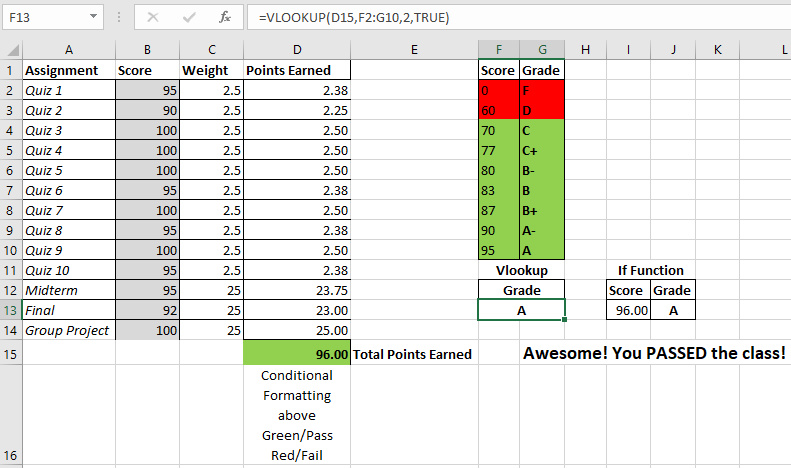
=VLOOKUP(D15,F2:G10,2,TRUE)
Values in Vlookup:
1. The first is the value we want to look up (lookup value)
2. Second is the range where the lookup value is.
Note: Lookup value should always be in the first column of the range
3. Third is the column of the range where the return value is located. In this case, we want the “Grade” which is column 2.
4. Lastly, TRUE for an approximate match and FALSE is for an exact match.
Note: TRUE is the default value
What Is Happening???
The VLookup Function is typed into cell F13 and automatically changes the grade based on the value of cell D15 (total points earned). Next, it uses the range F2 through G10 as the “grade key”. When it finds the matches the lookup value to the score, it returns the corresponding grade that’s in the 2nd column of the range F2:G10. Hopefully, it’s an A!
Try changing some of the scores in the gray background so you can see the VLookup do it’s job!
If Function Grade Based On Score
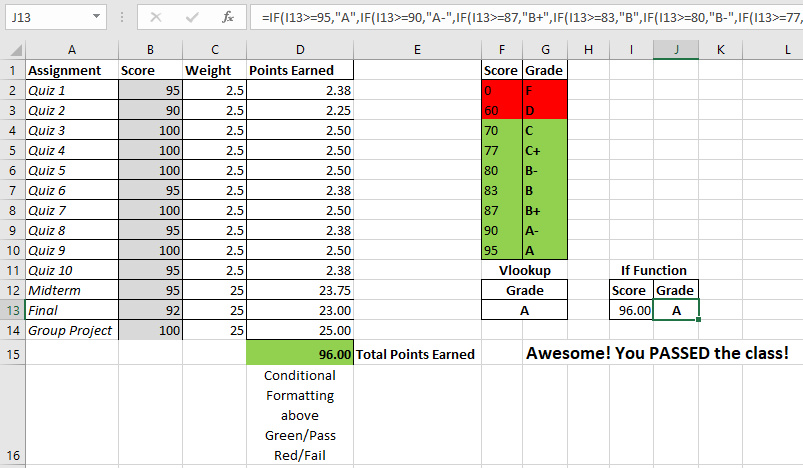
=IF(I13>=95,”A”,IF(I13>=90,”A-“,IF(I13>=87,”B+”,
IF(I13>=83,”B”,IF(I13>=80,”B-“,IF(I13>=77,”C+”,
IF(I13>=70,”C”,IF(I13>=60,”D”,”F”))))))))
This method of calculating your semester grade looks like more work, but it is actually easier as long as you are careful with your parenthesis. Just like math, if you open one you need to close it too. The “IF” function checks if the value is greater than or equal to 95. If that condition is true, it will display an “A”. If that condition is false, it will move to the next condition and so on. If none of the conditions are true, it will move to the default value. Sadly, the default value in this case is an “F”.
Again, try changing scores in the gray background so you can see the “IF” function in action!
Woah! Can I Have An Easier Example?!?
Yes! Your eyes may cross at first sight of the “IF” function above. I setup another “IF” function to print a motivational message base on the final grade.
=IF(D15>=70,”Awesome! You PASSED the class!”,”You FAILED! Better luck next year!”)
If the total points earned for the semester is greater than or equal to 70, then Excel will print “Awesome! You PASSED the class!”. If this condition is not met, total points earned are less than 70, and Excel will print “You FAILED! Better luck next year!”.
Awesome! You have learned to calculate your final semester grade with Vlookups, if functions, and conditional formatting.
About Me

A self-taught front end web developer who loves to travel, create things, solve problems, and grill! I enjoy the challenge of taking things apart, learning how they work, and improving them. I created this site to document and share what I've learned.